构建加密货币投资组合仪表盘是深入了解这个新兴金融市场的绝佳途径。与其他投资一样,它也存在一定的风险。因此,一旦创建了投资组合,持续跟踪其增长就变得至关重要。除了可视化随时间变化的趋势外,定期计算收益也有助于调整交易策略并做出市场入场和出场决策。
在今天的文章中,我们将探讨如何使用Observable Framework和 Python构建加密货币投资组合仪表盘。它将提供绝对和相对价格变化的全面细分,以及清晰的收益计算指标。由于加密货币市场全天候交易,我们还将使用 GitHub Actions 设置自动化功能,定期更新仪表盘。
以下是 仪表盘最终外观的实时预览,您可以点击此处访问Github 代码库 。让我们开始吧!

先决条件
除了 Python 3,我们还需要设置 Observable Framework,它是一个 Node.js 应用程序。请确保安装Node.js 18 或更高版本。此外,建议安装 yarn 作为包管理器。
npm install --global yarn
可以验证不同软件包的安装版本,如下所示:
节点--版本
npm --version
yarn --version
由于仪表板将作为 GitHub 页面托管,并使用 GitHub Actions 实现自动化,因此还需要个人 GitHub 帐户。
在 Observable 框架上创建新项目
我们将首先创建仪表板的文件夹结构。前端负责设计仪表板的外观,并将基于 JavaScript 编写。后端负责从 CoinGecko 获取历史价格数据,并将使用 Python 编写。要创建新项目,请运行:
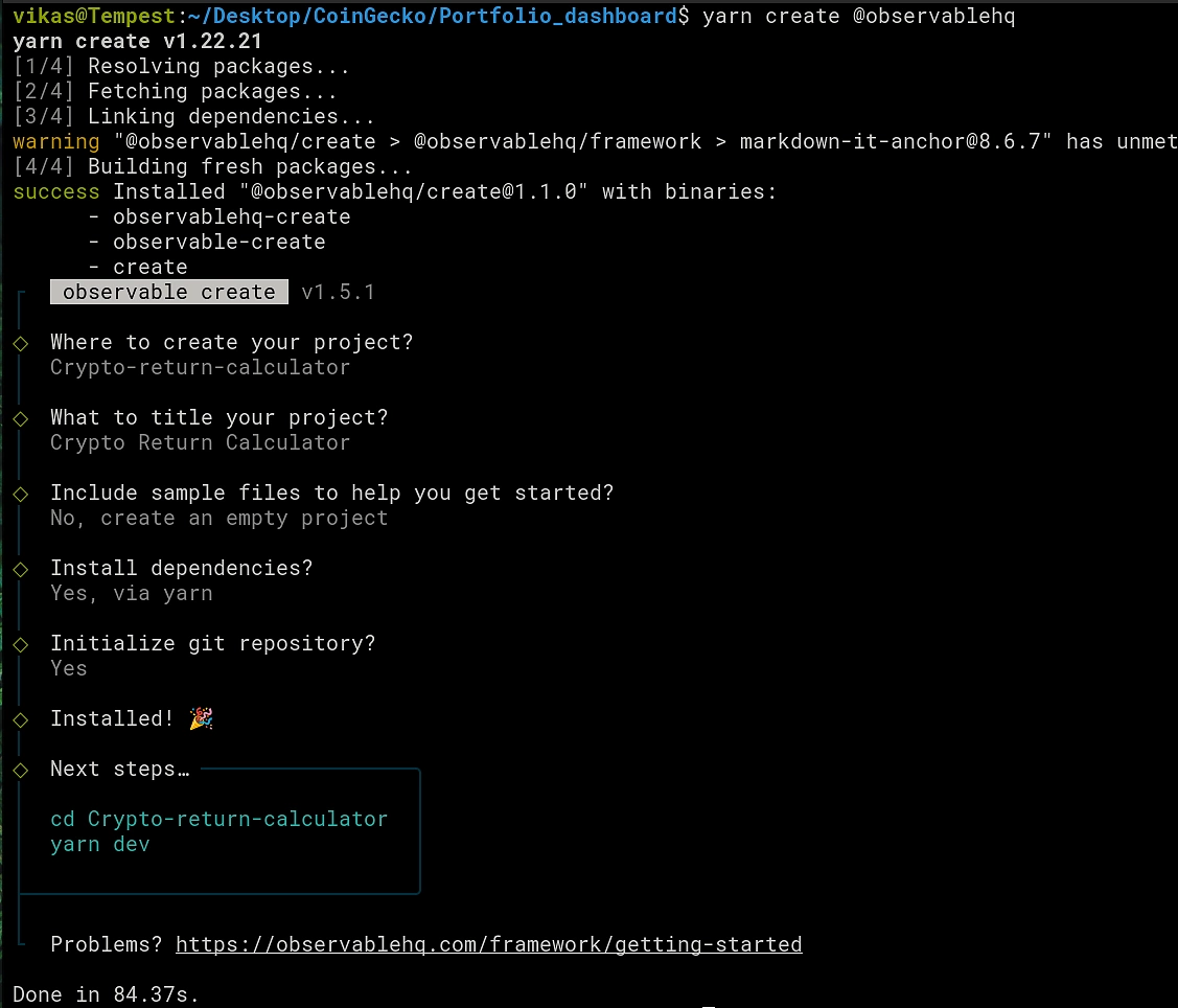
yarn create @observablehq
现在,将出现一系列提示,您可以根据自己的偏好进行回答。请注意,我们已选择 yarn 作为首选包管理器,并且还初始化了一个 git 仓库。
docs 文件夹将包含前端和后端的代码。在我们的例子中,Python 后端将用于向 CoinGecko 发出 API 调用并获取指定资产的历史价格数据。这也称为数据加载器,随后将由仪表板前端使用。在 docs 文件夹中,我们可以创建另一个文件夹 data 来存储所有 Python 代码。这将进一步有助于将代码组织到单独的文件中,以提高可读性,如下一节所示。
如何使用 API 获取历史硬币价格数据?
在文件中 api.py,我们定义了以下函数,用于从文件或环境变量本地读取 API 密钥。后者在使用 GitHub Actions 设置自动化时很重要,稍后将详细讨论。
| import requests as rq | |
| import json | |
| import os | |
| # Define a custom exception class | |
| class KeyNotFoundError(Exception): | |
| pass | |
| PRO_URL = "https://pro-api.coingecko.com/api/v3" | |
| # Get API key from file (when running locally) or from env. variable (during CI) | |
| def get_key(): | |
| file = "/home/vikas/Documents/CG_pro_key.json" | |
| if os.path.exists(file): | |
| f = open(file) | |
| key_dict = json.load(f) | |
| return key_dict["key"] | |
| else: | |
| key = os.getenv('CG_PRO_KEY') | |
| if key is not None: | |
| return key | |
| else: | |
| raise KeyNotFoundError("API key is not available!") |
现在我们定义另一个函数来处理 API 请求。响应代码 200 表示请求成功。
| use_pro = { | |
| "accept": "application/json", | |
| "x-cg-pro-api-key" : get_key() | |
| } | |
| def get_response(endpoint, headers, params, URL): | |
| url = "".join((URL, endpoint)) | |
| response = rq.get(url, headers = headers, params = params) | |
| if response.status_code == 200: | |
| data = response.json() | |
| return data | |
| else: | |
| print(f"Failed to fetch data, check status code {response.status_code}") |
| from api import get_response, PRO_URL, use_pro | |
| def get_hist_market(coin_id, currency, duration): | |
| params = { | |
| "vs_currency": currency, | |
| "days": duration, | |
| "precision": 2 | |
| } | |
| hist_data = get_response(f"/coins/{coin_id}/market_chart", | |
| use_pro, | |
| Params, | |
| PRO_URL) | |
| return hist_data |
# 天数
持续时间 = “120”
目标货币 = “eur”
# 定义投资组合
port_curr = [“bitcoin”, “ethereum”, “chainlink”, “dash”, “litecoin”]
port_amount = [0.10, 1.5, 300, 75, 50]
如何设置 Python 数据加载器?
数据加载器本质上是一个 Python 脚本(value.json.py),它执行以下操作:
-
获取给定硬币 ID 和指定持续时间的历史价格数据
-
创建包含每日价值(每日价格 x 投资组合金额)的细分词典
-
将字典转换为 JSON 并将数据转储到标准输出
| import json | |
| import sys | |
| from portfolio import duration, target_currency, port_amount, port_curr | |
| from data import get_hist_market | |
| from helpers import get_prices_dict, create_breakdown_dict | |
| breakdown_dict = None | |
| for (curr, amount) in zip(port_curr, port_amount): | |
| curr_hist = get_hist_market(curr, target_currency, duration) | |
| curr_dict = get_prices_dict(curr_hist["prices"]) | |
| # Correct for duplicate entry for latest date | |
| if len(curr_dict) > int(duration): | |
| curr_dict = curr_dict[0:int(duration)] | |
| if breakdown_dict is None: | |
| breakdown_dict = create_breakdown_dict(curr_dict, port_curr) | |
| for i in range(len(curr_dict)): | |
| daily_value = curr_dict[i]["price"] * amount | |
| breakdown_dict[i]["value"] += daily_value | |
| breakdown_dict[i][f"{curr}"] = daily_value | |
| json.dump(breakdown_dict, sys.stdout) |
| def get_prices_dict(prices): | |
| prices_dict = [] | |
| for i in range(len(prices)): | |
| # Convert to seconds | |
| s = prices[i][0] / 1000 | |
| prices_dict.append({'time' : datetime.datetime.fromtimestamp(s).strftime('%Y-%m-%d'), | |
| 'price' : prices[i][1]}) | |
| return prices_dict |
| def initialize_dict(port_curr): | |
| # Initialize dict with keys for all currencies | |
| port_value = [0.0 for i in range(len(port_curr))] | |
| breakdown = {port_curr[i] : port_value[i] for i in range(len(port_curr))} | |
| # Add key to store total value | |
| breakdown['value'] = 0.0 | |
| return breakdown | |
| def create_breakdown_dict(curr_dict, port_curr): | |
| # Create a list of dicts | |
| breakdown_dict = [] | |
| for i in range(len(curr_dict)): | |
| breakdown = initialize_dict(port_curr) | |
| breakdown['time'] = curr_dict[i]["time"] | |
| breakdown_dict.append(breakdown) | |
| return breakdown_dict |
如何设置你的加密货币投资组合仪表板
仪表板的页面被分组到 Markdown 文件中,其中可以使用特殊的代码块来执行 JavaScript 代码。主页内容在 index.md 文件中指定。此外,我们将按照以下思路创建另外两个页面:
-
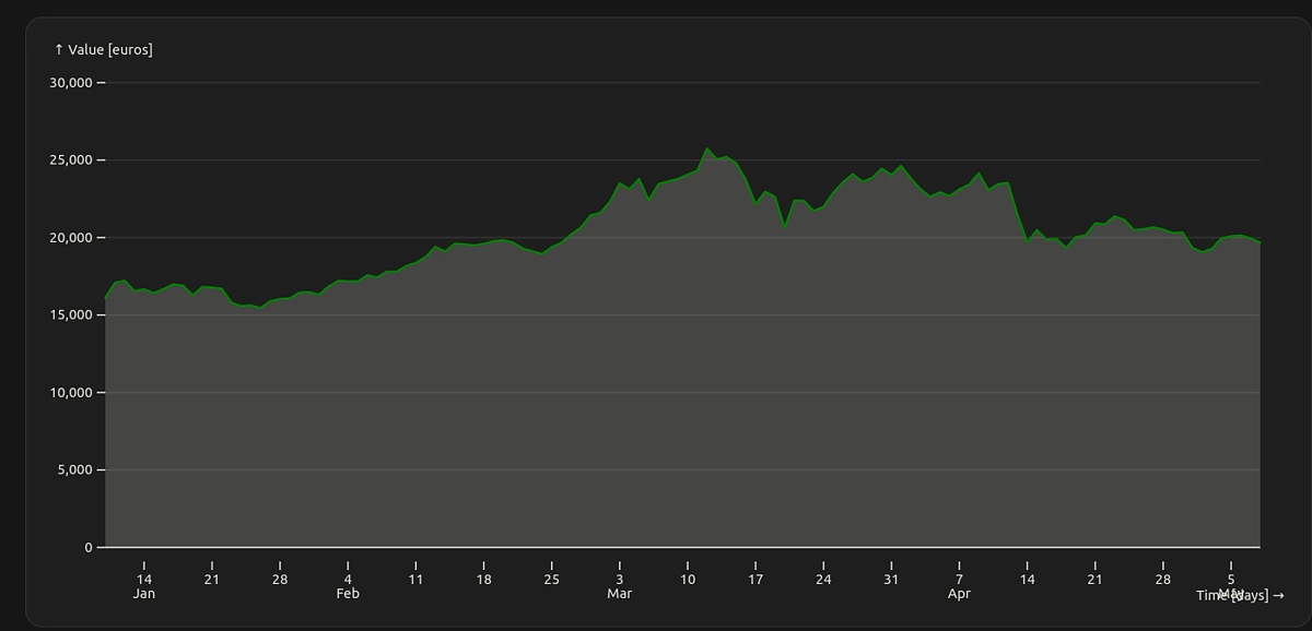
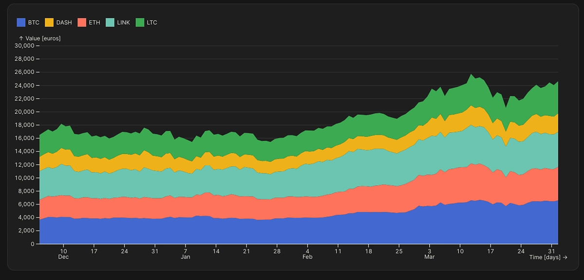
value.md - 显示投资组合总价值(欧元)的变化以及个别明细
-
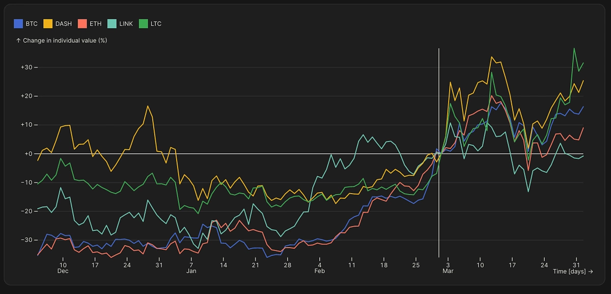
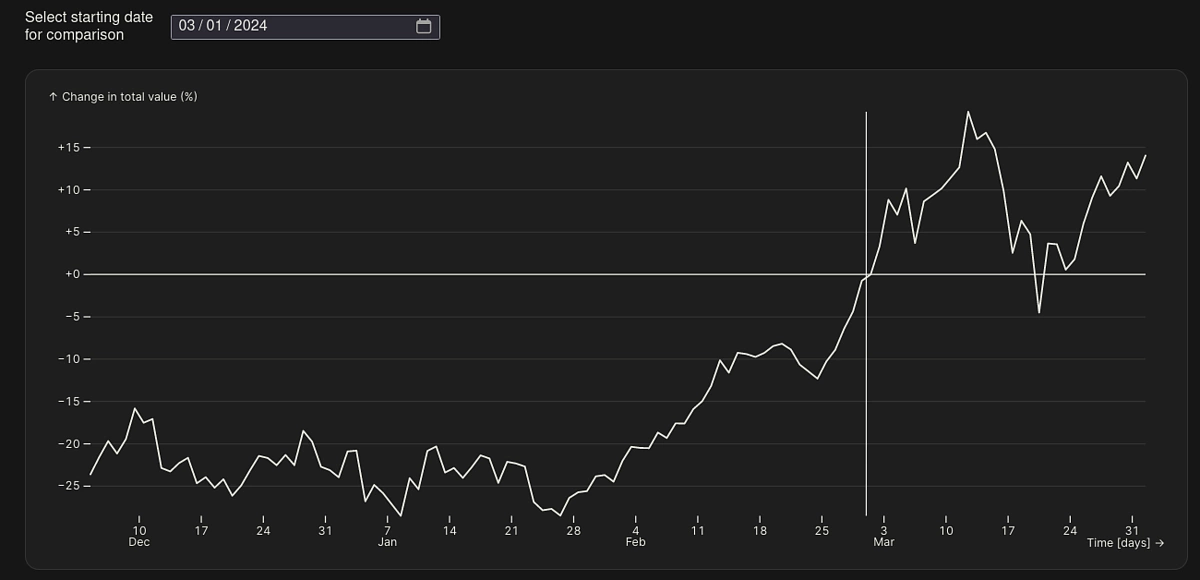
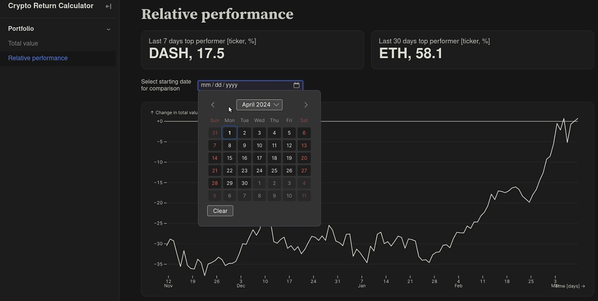
change.md - 通过交互式日期选择功能显示不同加密货币之间的相对变化(以%为单位)
与我们的 Python 后端类似,我们也可以将前端代码组织到单独的文件中,以便于复用和增强可读性。绘图函数分组放在 components/plots.js 文件中。对于第一页,我们想绘制一个线段+面积图来追踪投资组合的总价值变化。这可以使用强大的Observable Plot库来实现。
| import * as Plot from "npm:@observablehq/plot"; | |
| import * as d3 from "https://cdn.jsdelivr.net/npm/d3@7/+esm"; | |
| const domain_max = 30000 | |
| export function plotValue(breakdown, {width} = {}) { | |
| return Plot.plot({ | |
| width, | |
| //title: "Total portfolio value", | |
| x: {type: "utc", ticks: "week", label: "Time [days]"}, | |
| y: {grid: true, inset: 10, label: "Value [euros]", domain: [0, domain_max]}, | |
| marks: [ | |
| Plot.areaY(breakdown, { | |
| x: "time", | |
| y: "value", | |
| fillOpacity: 0.2 | |
| }), | |
| Plot.lineY(breakdown, { | |
| x: "time", | |
| y: "value", | |
| stroke: "green", | |
| tip: false | |
| }), | |
| Plot.ruleY([0]), | |
| Plot.ruleX(breakdown, Plot.pointerX({x: "time", | |
| py: "value", | |
| stroke: "red"})), | |
| Plot.dot(breakdown, Plot.pointerX({x: "time", | |
| y: "value", | |
| stroke: "red"})), | |
| Plot.text(breakdown, Plot.pointerX({px: "time", | |
| py: "value", | |
| dx: 100, | |
| dy: -18, | |
| frameAnchor: "top-left", | |
| fontVariant: "tabular-nums", | |
| text: (d) => [`Date ${d.time}`, | |
| `Value ${d.value.toFixed(2)}`].join(" ")})) | |
| ] | |
| }); | |
| } |
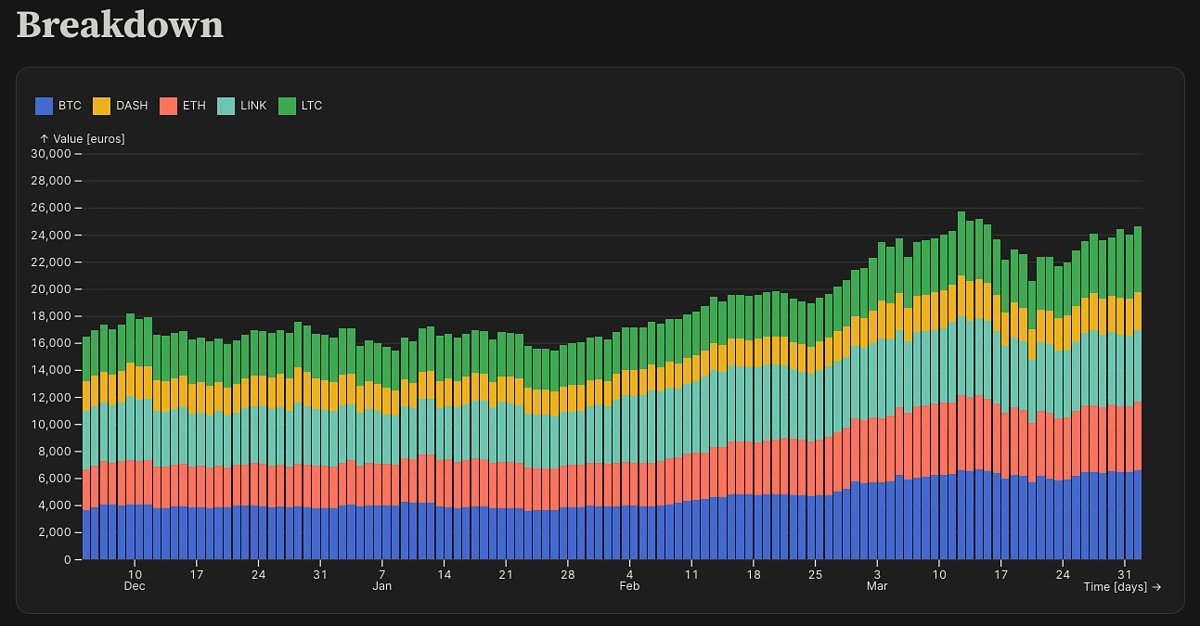
同样,它也有助于直观地展现投资组合中单个资产的变化,因为有些资产的价值可能会随着时间的推移保持不变或下降。因此,堆叠条形图是一种更深入地了解单个资产表现的简洁方法。
| export function plotBreakdownBar(stackArray, {width} = {}) { | |
| return Plot.plot({ | |
| width, | |
| //title: "Portfolio breakdown", | |
| x: {label: "Time [days]"}, | |
| y: {grid: true, label: "Value [euros]", domain: [0, domain_max]}, | |
| color: {legend: true}, | |
| marks: [ | |
| Plot.rectY(stackArray, { | |
| x: "time", | |
| y: "value", | |
| interval: "day", | |
| fill: "name", | |
| tip: true | |
| }) | |
| ] | |
| }); | |
| } |
堆积面积图显示相同的信息,但更具视觉吸引力。
| export function plotBreakdownArea(stackArray, {width} = {}) { | |
| return Plot.plot({ | |
| width, | |
| //title: "Portfolio breakdown", | |
| x: {label: "Time [days]"}, | |
| y: {grid: true, label: "Value [euros]", domain: [0, domain_max]}, | |
| color: {legend: true}, | |
| marks: [ | |
| Plot.areaY(stackArray, { | |
| x: "time", | |
| y: "value", | |
| interval: "day", | |
| fill: "name", | |
| tip: true | |
| }), | |
| Plot.ruleY([0]) | |
| ] | |
| }); | |
| } |
为了让用户更好地了解投资组合变化的幅度,我们还可以在顶行添加两张卡片,一张显示过去 7 天的百分比变化,另一张显示过去 30 天的百分比变化。
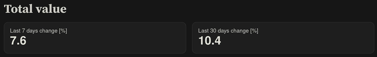
可以通过创建 JavaScript 函数 getPertChange 轻松计算出百分比变化,该函数以天数作为附加输入。
| export function getPertChange(breakdown, num_days) { | |
| const change = (breakdown[breakdown.length - 1].value - | |
| breakdown[breakdown.length - 1 - num_days].value) | |
| / breakdown[breakdown.length - 1- num_days].value | |
| // Change % | |
| const pert_change = change * 100; | |
| // Round off to first digit after decimal | |
| return Math.round(pert_change * 10) / 10 | |
| } |
页面的整体布局通过 value.md 中的以下代码控制:
| theme | toc |
|---|---|
|
dashboard
|
false
|
Total value
import {plotValue, plotBreakdownBar, plotBreakdownArea} from "./components/plots.js";import {createStack, getPertChange} from "./components/helpers.js";
const breakdown = FileAttachment("./data/value.json").json();
Last 7 days change [%]
Last 30 days change [%]
Breakdown
第二页(change.md)显示了比较投资组合中所有资产时的相对表现。
| export function plotBreakdownChange(stackArray, date, {width} = {}) { | |
| const bisector = d3.bisector((i) => stackArray[i].time); | |
| const basis = (I, Y) => Y[I[bisector.center(I, date)]]; | |
| return Plot.plot({ | |
| style: "overflow: visible;", | |
| y: { | |
| //type: "log", | |
| grid: true, | |
| label: "Change in individual value (%)", | |
| tickFormat: ((f) => (x) => f((x - 1) * 100))(d3.format("+d")), | |
| //domain: [0, 100] | |
| }, | |
| width, | |
| //title: "", | |
| x: {label: "Time [days]"}, | |
| color: {legend: true}, | |
| marks: [ | |
| Plot.ruleY([1]), | |
| Plot.ruleX([date]), | |
| Plot.lineY(stackArray, Plot.normalizeY(basis, { | |
| x: "time", | |
| y: "value", | |
| interval: "day", | |
| stroke: "name", | |
| //marker: true | |
| //tip: true | |
| })), | |
| ] | |
| }); | |
| } |
可以采取类似的方法来显示总价值的变化。
| export function plotValueChange(breakdown, date, {width} = {}) { | |
| const bisector = d3.bisector((i) => breakdown[i].time); | |
| const basis = (I, Y) => Y[I[bisector.center(I, date)]]; | |
| return Plot.plot({ | |
| style: "overflow: visible;", | |
| y: { | |
| //type: "log", | |
| grid: true, | |
| label: "Change in total value (%)", | |
| tickFormat: ((f) => (x) => f((x - 1) * 100))(d3.format("+d")), | |
| //domain: [0, 100] | |
| }, | |
| width, | |
| //title: "", | |
| x: {label: "Time [days]"}, | |
| color: {legend: true}, | |
| marks: [ | |
| Plot.ruleY([1]), | |
| Plot.ruleX([date]), | |
| Plot.lineY(breakdown, Plot.normalizeY(basis, { | |
| x: "time", | |
| y: "value", | |
| interval: "day", | |
| //stroke: "name", | |
| //marker: true | |
| //tip: true | |
| })), | |
| ] | |
| }); | |
| } |
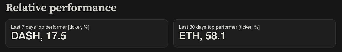
与第一页类似,在顶部添加两张卡片会很有用,显示 7 天和 30 天内表现最佳的商品(价值变化的最大百分比)。
 为了计算出表现最佳者,我们利用以下逻辑:
| export function getTopPerformer(breakdown, num_days) { | |
| const changeArray = [] | |
| for (let i = 0; i < names.length; i++) { | |
| const changeObj = { | |
| name: names[i], | |
| change: (breakdown[breakdown.length - 1][names[i]] - | |
| breakdown[breakdown.length - 1 - num_days][names[i]]) | |
| / breakdown[breakdown.length - 1- num_days][names[i]] | |
| } | |
| changeArray.push(changeObj) | |
| } | |
| // Find maximum value and its corresponding index in changeArray | |
| let maxValue = -Infinity; | |
| let maxIndex = -1; | |
| for (let i = 0; i < changeArray.length; i++) { | |
| if (changeArray[i].change > maxValue) { | |
| maxValue = changeArray[i].change; | |
| maxIndex = i; | |
| } | |
| } | |
| // Change % | |
| const maxChange = maxValue * 100; | |
| // Round off to first digit after decimal | |
| const roundMaxChange = Math.round(maxChange * 10) / 10; | |
| const resultObj = { | |
| maxChange: roundMaxChange, | |
| maxName: tickers[maxIndex] | |
| } | |
| return resultObj | |
| } |
|
const date = view( |
整体页面布局通过以下逻辑控制:
| theme | toc |
|---|---|
|
dashboard
|
false
|
Relative performance
import {plotBreakdownChange, plotValueChange} from "./components/plots.js";import {createClubbedStack, convertDates, getTopPerformer} from "./components/helpers.js";import * as Inputs from "npm:@observablehq/inputs";
const breakdown = FileAttachment("./data/value.json").json();
const weeklyObj = getTopPerformer(breakdown, 7);const monthlyObj = getTopPerformer(breakdown, 30);
Last 7 days top performer [ticker, %]
Last 30 days top performer [ticker, %]
const clubbedStack = createClubbedStack(breakdown)
const date = view( Inputs.date({ label: "Select starting date for comparison", min: clubbedStack[0].time, max: clubbedStack[clubbedStack.length - 1].time }));
如何在本地测试仪表板?
前后端代码准备就绪后,即可在本地构建仪表板,以验证一切是否按预期运行。Observable Framework 支持实时预览,这意味着每当发生任何更改时,浏览器内页面都会自动更新。这有助于快速测试对页面布局或数据加载器所做的任何更改的影响。
要启动预览服务器,请执行以下操作:
纱线开发
浏览器窗口应该会自动打开。如果没有,请访问以下地址: http://127.0.0.1:3000/
如何将仪表板部署到 GitHub Pages?
在上一节中,我们设法在本地生成仪表板。
由于您可能还想在远离笔记本电脑或手机时查看您的投资组合,我们现在将更进一步,利用 GitHub Actions 将我们的仪表板自动部署到我们自己的 GitHub 页面 - 这将使其可在所有设备上访问。
我们甚至可以设置仪表板更新的时间表,以确保任何突然的价格变动的影响都能立即被我们看到。
Observable 项目最初被初始化为 Git 仓库。现在可以将其推送到 GitHub,就像本文中对代码所做的那样。现在我们需要为 Pages 启用部署功能。前往“设置” > “页面” > “构建和部署” > “源”(选择“GitHub 操作”)。
CoinGecko API 密钥应保存为存储库密钥:设置>密钥和变量>操作>密钥 > 存储库密钥>新存储库密钥。
下一步是创建一个用于构建和部署仪表板的工作流文件。该文件包含一个或多个作业,这些作业本质上是一系列步骤,描述了我们如何创建软件环境和构建仪表板。我们需要确保在构建作业期间首先安装所有依赖项(Node.js 和 Python)。最后一步是上传工件,这些工件将由部署作业获取,部署作业详细说明了页面的创建方式。
| name: Deploy to GitHub pages | |
| on: | |
| push: | |
| branches: [ main ] | |
| pull_request: | |
| branches: ["main"] | |
| schedule: | |
| - cron: "30 */2 * * *" | |
| jobs: | |
| build: | |
| runs-on: ubuntu-latest | |
| env: | |
| CG_PRO_KEY: ${{ secrets.CG_PRO_KEY }} | |
| permissions: | |
| contents: write | |
| deployments: write | |
| id-token: write | |
| packages: read | |
| steps: | |
| - uses: actions/checkout@v4 | |
| - uses: actions/setup-node@v4 | |
| with: | |
| node-version: 20 | |
| cache: 'yarn' | |
| cache-dependency-path: yarn.lock | |
| - run: yarn --frozen-lockfile | |
| # This step will generate the build data in dist folder | |
| - name: Build website | |
| run: yarn build | |
| - name: Upload Pages artifact | |
| uses: actions/upload-pages-artifact@v3 | |
| with: | |
| path: "dist/" | |
| deploy: | |
| # Add a dependency to the build job | |
| needs: build | |
| # Grant GITHUB_TOKEN the permissions required to make a Pages deployment | |
| permissions: | |
| pages: write # to deploy to Pages | |
| id-token: write # to verify the deployment originates from an appropriate source | |
| # Deploy to the github-pages environment | |
| environment: | |
| name: github-pages | |
| url: ${{ steps.deployment.outputs.page_url }} | |
| # Specify runner + deployment step | |
| runs-on: ubuntu-latest | |
| steps: | |
| - name: Deploy to GitHub Pages | |
| id: deployment | |
| uses: actions/deploy-pages@v4 |
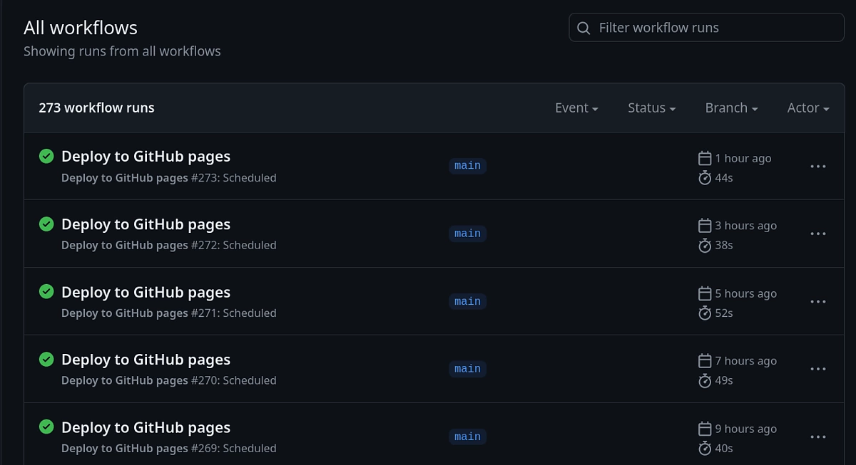
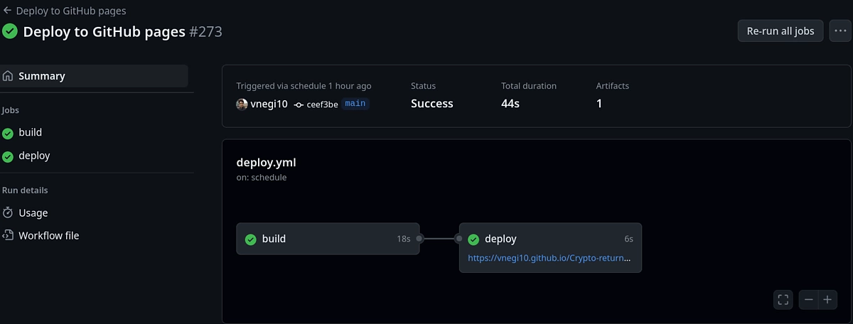
打开单个工作流结果会显示一个包含所有已连接作业(本例中仅包含两个)的图表。已部署的 GitHub 页面的 URL 也可见。
💡 专业提示:默认情况下,GitHub 页面对所有人可见。如果您希望私下发布网站,则需要创建组织帐户并使用企业云。
要检查您的投资组合健康状况,您现在可以将仪表板 URL 添加到书签,并随时访问它!